Delving Deeper into Convolutional Networks for Learning Video Representations

• Paper summary
• Delving Deeper into Convolutional Networks for Learning Video Representations Ballas et al. (2016)
• Nicolas Ballas, Li Yao, Chris Pal, and Aaron Courville

1. Introduction

• Video analysis and understanding
  • Human action recognition, video retrieval or video captioning
  • Previous: hand-crafted and task-specific representations
• Current researches
  • CNN: image analysis (good) but NOT use temporal information
  • RNN: temporal sequences analysis (good)
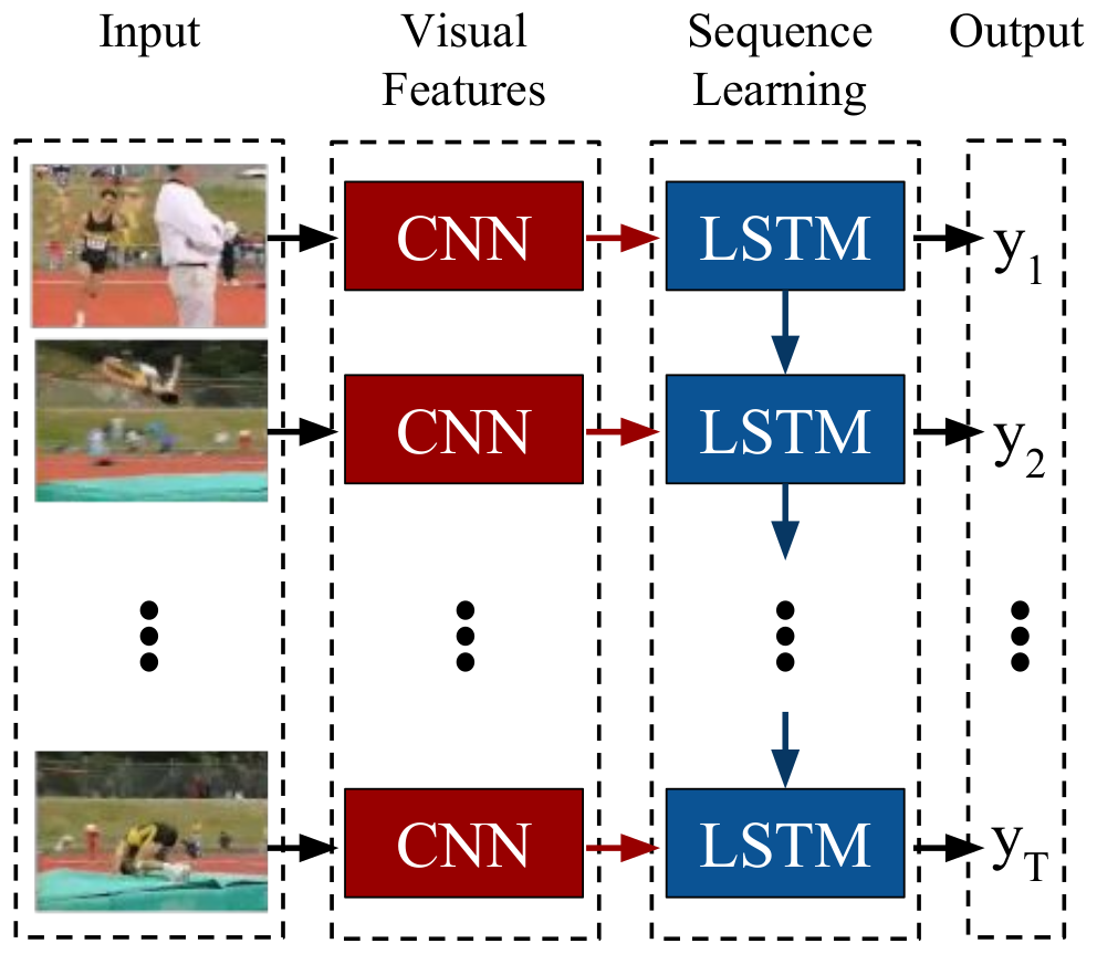
• Recurrent Convolutional Networks (RCN)
  • Srivastava et al. (2015) ¹; Donahue et al. (2014) ²; Ng et al., 2015 ³
  • RNN + CNN for learning video representations

Recurrent Convolutional Networks (RCN)

• Basic architecture
  • Visual percepts: CNN feature maps
  • RNN input: Visual percepts
• Previous works
  • High-level visual percepts (only top-layer)
  • Drawbacks: local information을 많이 잃어버림
  • Drawbacks: frame-to-frame에서 temporal variation이 크지 않음
• Novel architecture
  • top-layer + middle-layers
  • GRU-RNN: conv2d ops instead of fc ops in RNN cell

2. Gated Recurrent Unit Networks (GRU)

• Learning phrase representations using rnn encoder-decoder for statistical machine translation, Cho et. al. (2014) ⁴
  • long-term temporal dependency modelling
  • ${\bf z}_{t}$: update gate
  • ${\bf r}_{t}$: reset gate
  • $\odot$: element-wise multiplication

3. Delving Deeper into Convolutional Neural Networks

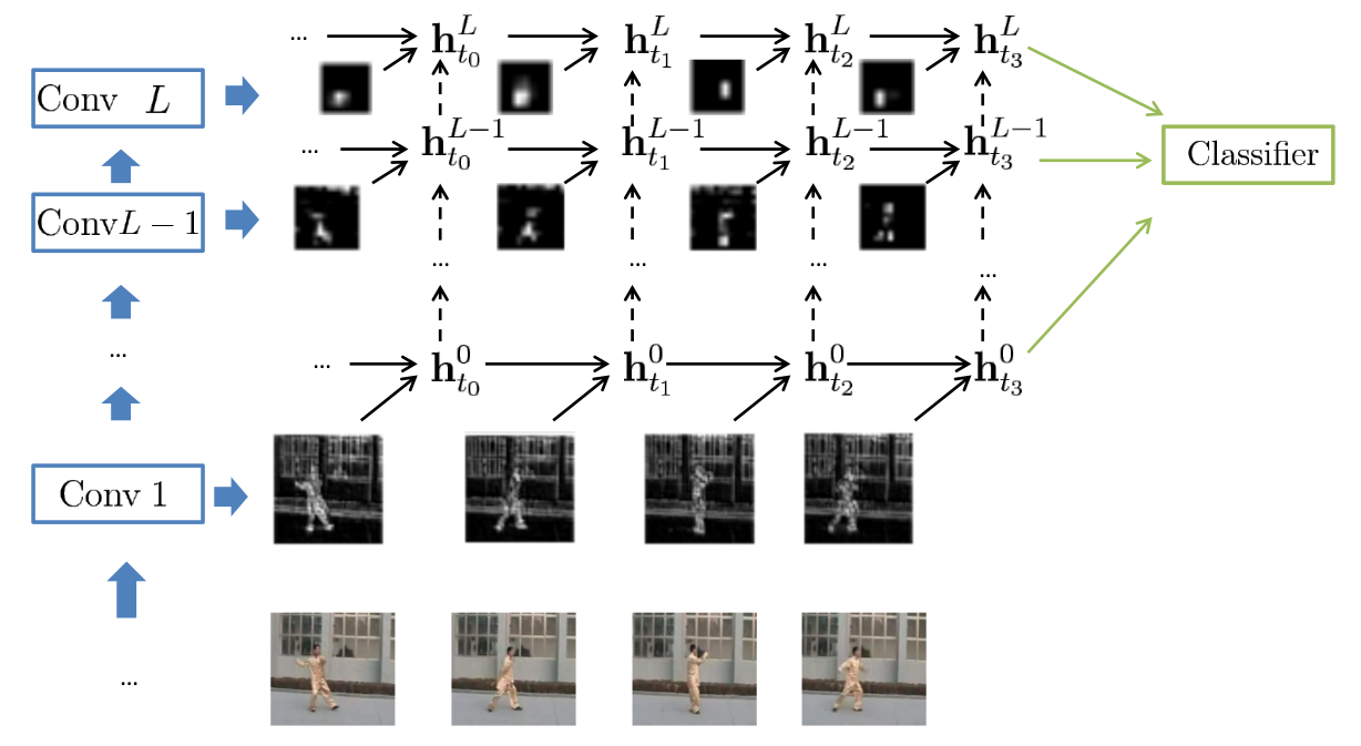
Two GRU-RCN architectures

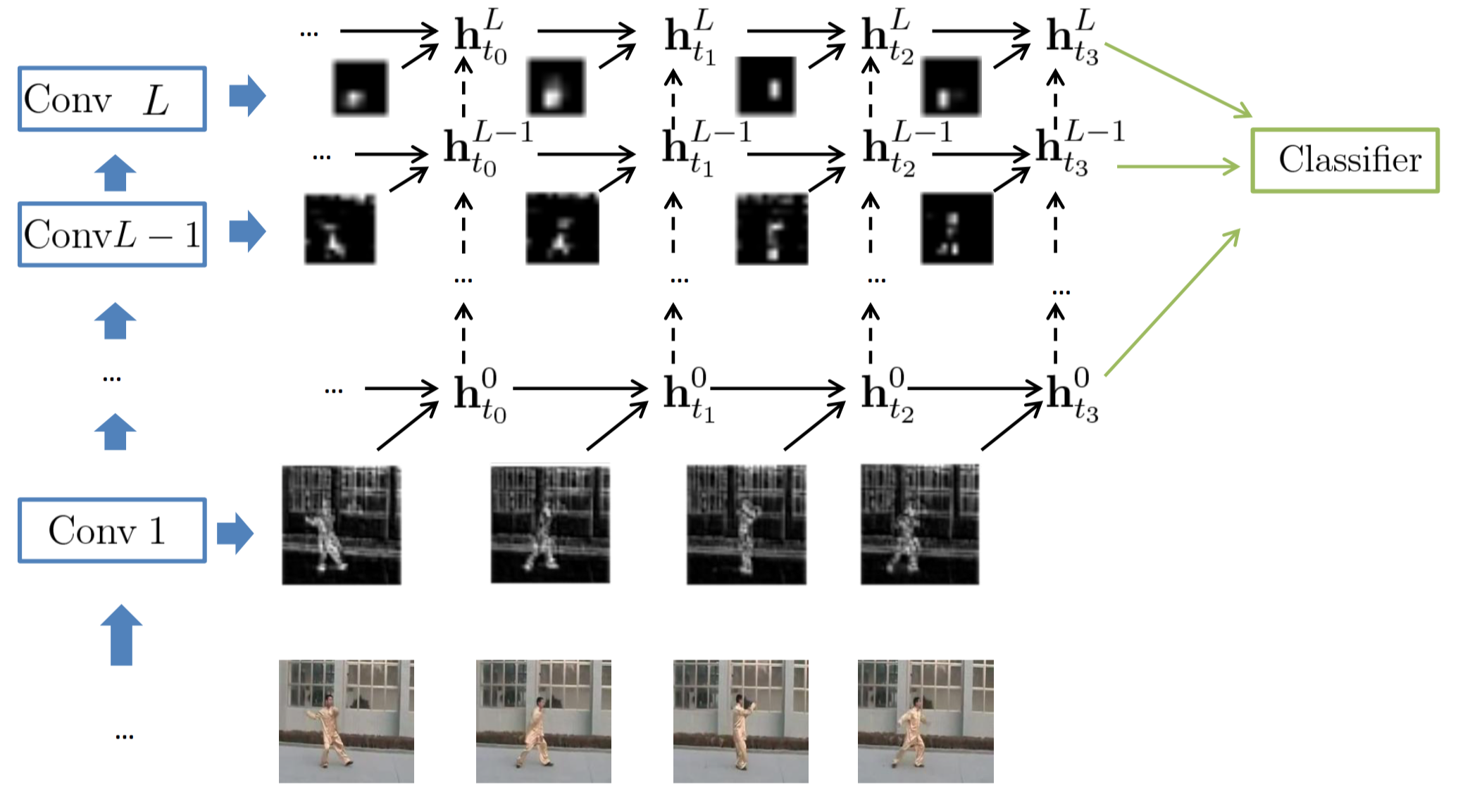
• GRU-RCN (그림에서 위 방향 점선 화살표를 빼면 됨)
• Stacked GRU-RCN (figure)
• $ (\mathbf{x}_{t}^{1}, \cdots, \mathbf{x}_t^{L-1}, \mathbf{x}_t^{L}) $
  • $t=1, \cdots, T$

3.1 GRU-RCN

• $ \mathbf{h}_t^l$ $= \phi^l(\mathbf{x}_t^l,$ $\mathbf{h}_{t-1}^{l})$
• $*$: conv2d ops
• 맨 마지막 시점의 hidden들$(\mathbf{h}_{T}^{1}, \cdots, \mathbf{h}_T^{L})$을 가지고 classify
• fc ops: conv maps의 특성을 반영하지 못함
• conv maps: 다른 위치에서 반복적으로 나타나는 강한 local correlation을 끄집어냄

number of parameters

• number of parameters in GRU
  • Size of $\mathbf{W}^{l}$, $\mathbf{W}_{z}^{l}$ and $\mathbf{W}_{r}^{l}$:
    • $N_{1} \times N_{2} \times O_{x} \times O_{h}$
    • $N$: input spatial size, $O_{x}$: input channels, $O_{h}$: size of hidden node
• number of parameters in GRU-RCN
  • Size of $\mathbf{W}^{l}$, $\mathbf{W}_{z}^{l}$ and $\mathbf{W}_{r}^{l}$:
    • $k_{1} \times k_{2} \times O_{x} \times O_{h}$
    • $k$: kernel size; usually $3 \times 3 \ll N_{1} \times N_{2}$

3.2 Stacked GRU-RCN

• $\mathbf{h}_{t}^{l}$ $= \phi^{l}(\mathbf{x}_{t}^{l},$ $\mathbf{h}_{t-1}^{l},$ $\mathbf{h}_{t}^{l-1})$
  • add $\mathbf{h}_{t}^{l-1}$: current time step and previous layer
• $*$: conv2d ops

4. Related Works

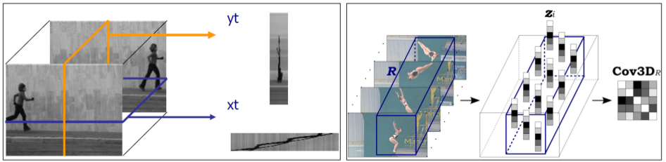
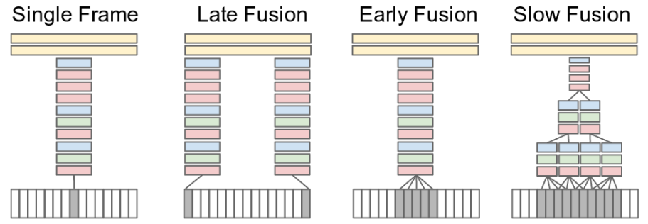
• Large-scale Video Classification with Convolutional Neural Networks Karpathy et al. (2014) ⁵
• C3D Tran et al. (2015) ⁶
• 이미지 분류와 달리 비약적인 발전은 없었음
• 오히려 큰 데이터 셋으로 비디오 학습은 힘들다고 함
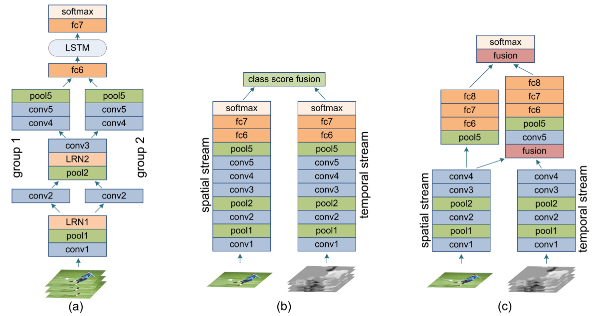
• Two-stream network Simonyan and Zisserman (2014) ⁷
• RGB color와 optical flow 정보를 각각 인풋으로 넣고 CNN 학습함
• Donahue et al. (2014) ², Ng et al., 2015 ³: Two-stream framework모델의 top layer를 RNN 적용

5. Experiments

5.1 Action Recognition

5.1.1 Model Architecture

• VGG-16: (ImageNet pertained $\rightarrow$ UCF-101로 fine tuning)
• extract 5 feature maps: pool2, pool3, pool4, pool5, and fc-7
• 위의 feature map들이 RCN 모델의 ${\bf x}_{t}^{l}$ input
  • $\mathbf{x}_{t}^{1}$: pool2
  • $\mathbf{x}_{t}^{2}$: pool3
  • $\vdots$
  • $\mathbf{x}_{t}^{5}$: fc-7
• UCF-101 dataset
  • 101 action, 13320 youtube video clips

Three RCN architectures

1. GRU-RCN
   • number of feature maps: 64, 128, 256, 256, 512
   • average pooling in last time step $T$
   • ex) Layer 1: pool2 (56 x 56 x 64) $\rightarrow$ (1 x 1 x 64)로 바꿔주기 위함
   • 각각을 다섯개의 classifier로 보냄
   • 한 classifier는 하나의 hidden representation에만 focus를 맞추고 학습
   • 최종 결정은 다섯개의 classifier average로 결정
   • dropout prob: 0.7
2. Stacked GRU-RCN
   • bottom-up connection이 얼마나 중요한지 조사하기 위해 실험
   • 아래 layer input의 spatial dimension을 맞추기 위해 max-pooling을 함
3. Bi-directional GRU-RCN
   • reverse temporal information의 중요성을 체크하기 위해 실험

5.1.2 Model Training and Evaluation

• Follow the two-stream framework
• batch size: 64 videos
• 네가지 사이즈 256, 224, 192, 168 중 하나로 random하게 cropping
• temporal cropping size: 10
• 최종 인풋은 224로 resize, 최종 인풋의 볼륨은 (224 x 224 x 10)
• Maximum log-likelihood

5.1.3 Results

Baseline result

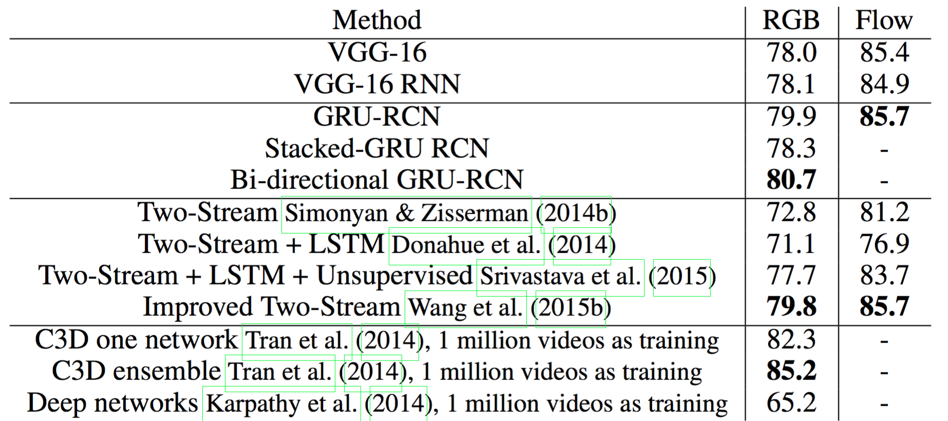
• VGG-16: pre-trained ImageNet and fine tune on the UCF-101
• VGG-16 RNN: fc-7을 GRU의 input 으로 넣음
  • GRU cell이 fully connected
• VGG-16 RNN(78.1) $>$ VGG-16(78.0): slightly improve
• CNN top-layer가 temporal information을 많이 잃어버렸다는 증거

RGB test

• Best: Bi-directional GRU-RCN
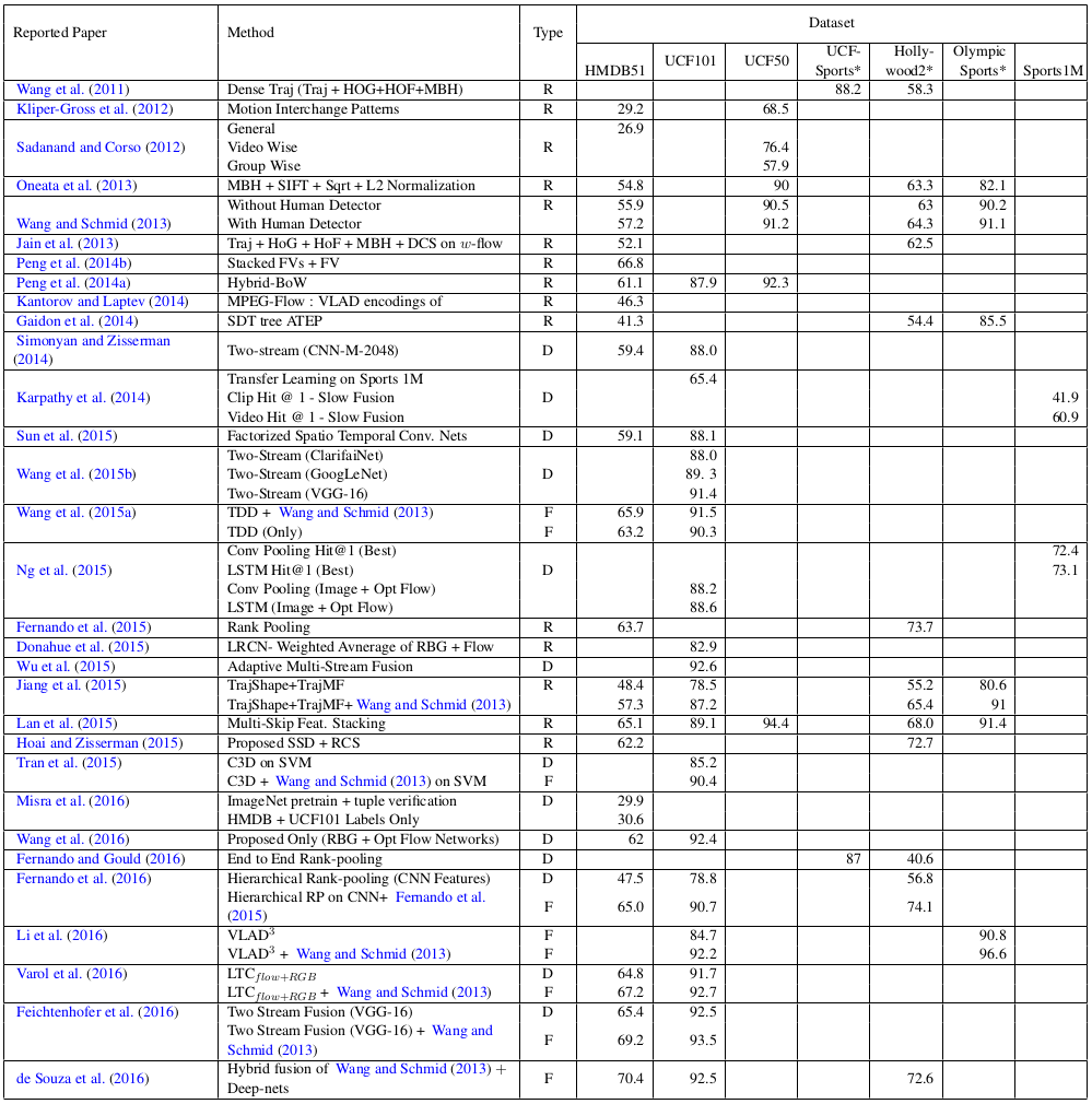
• state-of-art
  • C3D (Tran et. al.): 85.2
  • Karpathy: 65.2

Flow test

• Best: GRU-RCN (85.4 $\rightarrow$ 85.7)
• VGG16이 이미 10장의 연속된 이미지를 가지고 학습하기 때문에 그런 것 같음

RGB + Flow

• Details: Wang et al., (2015b) ⁸
• 두 모델을 각각 돌리고 weighted linear combination
• baseline: fusion VGG-16: 89.1; state-of-art: 90.9 (Wang)
• Combining Bi-directional GRU-RCN: 90.8

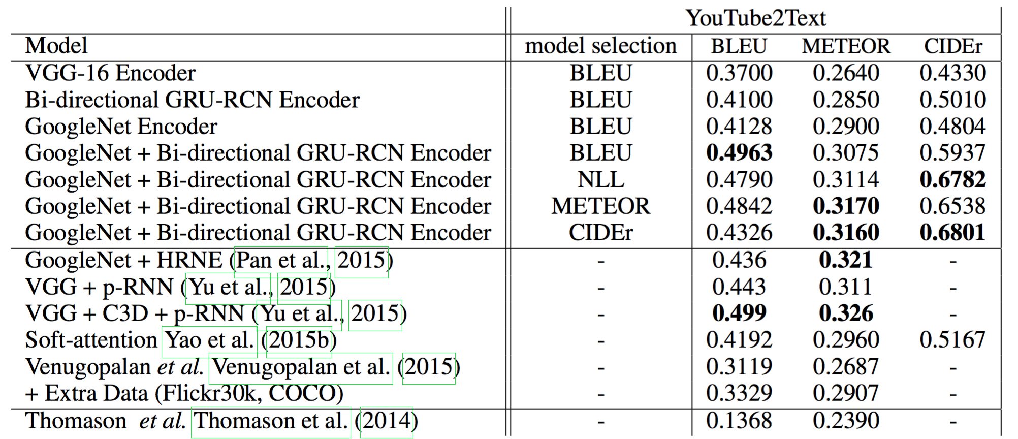
5.2 Video Captioning

5.2.1 Model Specifications

• Data
  • YouTube2Text: 1970 video clips with multiple natural language descriptions
  • train: 1200, valid: 100, test: 670
• Encoder-decoder framework: Cho et. al. (2014) ⁴
• Encoder
  • K equally-space segments(K=10)
  • 10개로 segment를 나누고 각각의 VGG-16에서 fc7 layer를 뽑아냄
  • 마지막 time step에서 합치고 (concatenate) 그걸 input 으로 사용
• Decoder: LSTM text-generator with soft-attention, Yao et. al. (2015b) ⁹

5.2.2 Training

5.2.3 Results

6. Conclusion

• temporal variation을 잘 모델링하기 위해 서로 다른 spatial resolution을 이용
• top layer에 가까우면 discriminative information이 더 높지만 spatial resolution이 떨어짐
• 아래 레이어에 가까우면 그 반대
• VGG-16에서 5개의 layer를 뽑아 멀티 레벨 GRU 적용

Miscellaneous

• 발표자료다운
• 모두의 연구소 자료 링크

References

Self-Normalizing Neural Networks

• Paper summary
• Self-Normalizing Neural Networks Klambauer et al. (2017)
• Günter Klambauer, Thomas Unterthiner, Andreas Mayr and Sepp Hochreiter

Abstract

• Success of Standard feed-forward neural networks(FNN) is rare
  • FNN cannot exploit many levels of abstract representations
• Self-normalizing neural networks
  • enable high-level abstract representations
  • Scaled exponential linear units (SELUs)
  • Banach fixed-point theorem
    • activations will converge toward zero mean and unit variance
    • vanishing and exploding gradients are impossible
    • Github link

Introduction

• Deep learning has very success
  • CNN: vision and video task
    • self-driving, AlphaGo
    • Kaggle: the “Diabetic Retinopathy” and the “Right Whale” challenge
  • RNN: speech and natural language processing
• Kaggle challenges that are not related to vision or sequential tasks
  • gradient boosting, random forests, SVMs are winning
  • very few cases where FNNs won, which are almost shallow
  • winning using FNN with at most 4 hidden layers
    • HIGGS challenge
    • Merck Molecular Activity challenge
    • Tox21 Data challenge
• Various normalization
  • Batch normalization Ioffe et al. (2016) ¹
  • Layer normalization Ba et al. (2016) ²
  • Weight normalization Salimans et al. (2016) ³
• Training with normalization techniques is perturbed by
  • SGD, stochastic regularization (like dropout), the estimation of the normalization parameters
• RNNs, CNNs can stabilize learning via weight sharing
• FNNs trained with normalization suffer from these perturbations and have high variance in the training error
  • This high variance hinders learning and slows it down
  • Authors believe this sensitivity to perturbations is the reason that FNNs are less successful than RNNs and CNNs

Figure 1. The training error (y-axis) on left: MNIST, right: CIFAR-10. FNN with bn exhibit high variance due to perturbations.

Self-Normalizing Neural Networks (SNNs)

Normalization and SNNs

• activation function: $f$
• weight matrix: $\bf{W}$
• activations in the lower layer: $\bf{x}$
• network inputs: $\mathbf{z} = \mathbf{W} \mathbf{x}$
• activations in the higher layer: $\mathbf{y} = f(\mathbf{z})$
• activations $\bf{x}, \bf{y}$ and inputs $\bf{z}$ are random variables

Assume

• all activations $x_{i}$
  • mean $\mu := \mathbb{E}(x_{i})$ across samples
    • $\mathbb{E} := \sum^{N}$: $N$ is a sample size (my notation)
  • variance $\nu := \textrm{Var}(x_{i})$
• That means
  • $\mu := \mathbb{E}(x_{1}) = \mathbb{E}(x_{2}) = \cdots = \mathbb{E}(x_{n})$
  • $\nu := \textrm{Var}(x_{1}) = \textrm{Var}(x_{2}) = \cdots = \textrm{Var}(x_{n})$
  • $\mathbf{x} = (x_{1}, x_{2}, \cdots, x_{n})$
• single activation $y = f(z), z = \mathbf{w}^{T} \mathbf{x}$
  • mean $\tilde{\mu} := \mathbb{E}(y)$
  • variance $\tilde{\nu} := \textrm{Var}(y)$

Define

• $n$ times the mean of the weight vector
  • $\omega := \sum_{i=1}^{n} w_{i}$, for $\mathbf{w} \in \mathbb{R}^{n}$
• $n$ times the second moment of the weight vector
  • $\tau := \sum_{i=1}^{n} w_{i}^{2}$, for $\mathbf{w} \in \mathbb{R}^{n}$

mapping $g$

$\left( \begin{array}{c} \mu \\ \nu \end{array} \right) \mapsto \left( \begin{array}{c} \tilde{\mu} \\ \tilde{\nu} \end{array} \right) \quad : \quad \left( \begin{array}{c} \tilde{\mu} \\ \tilde{\nu} \end{array} \right) = g \left( \begin{array}{c} \mu \\ \nu \end{array} \right)$

• mapping $g$ keeps $(\mu, \nu)$ and $(\tilde{\mu}, \tilde{\nu})$ close to predefined values, typically $(0, 1)$
  • like most normalization techniques: batch, layer, or weight normalization

Notation summary

• relate to activations: $(\mu, \nu, \tilde{\mu}, \tilde{\nu})$
• relate to weight : $(\omega, \tau)$

Definition 1 (Self-normalizing neural net)

A neural network is self-normalizing if it possesses a mapping $g : \Omega \mapsto \Omega$ for each activation $y$ that maps mean and variance from one layer to the next and has a stable and attracting fixed point depending on $(\omega, \tau)$ in $\Omega$. Furthermore, the mean and the variance remain in the domain $\Omega$, that is $g(\Omega) \subseteq \Omega$, where $\Omega = {(\mu, \nu) | \mu \in [\mu_{\textrm{min}}, \mu_{\textrm{max}}], \nu \in [\nu_{\textrm{min}}, \nu_{\textrm{max}}]}$. When iteratively applying the mapping $g$, each point within $\Omega$ converges to this fixed point.

• if both their mean and their variance across samples are within predefined intervals
  • then activations are normalized.

Constructing Self-normalizing Neural Networks

• Tow design choices
  1. the activation function
  2. the initialization of the weight

Scaled exponential linear units (SELUs)

$\textrm{selu}(x) = \lambda \left\{ \begin{array}{ll} x & \textrm{if} \ x > 0 \\ \alpha e^{x} - \alpha & \textrm{if} \ x \leq 0 \end{array} \right.$

1. negative and positive values for controlling the mean
2. saturation regions (derivatives approaching zero) to dampen the variance if it is too large in the lower layer
3. a slope larger than one to increase the variance if it is too small in the lower layer
4. a continuous curve.

Weight initialization

• propose $\omega = 0$ and $\tau = 1$ for all units in the higher layer

Deriving the Mean and Variance Mapping Function $g$

Assume

• $x_{i}$: independent from each other but share the same mean $\mu$ and variance $\nu$
  • $\mu := \mathbb{E}(x_{1}) = \mathbb{E}(x_{2}) = \cdots = \mathbb{E}(x_{n})$
  • $\nu := \textrm{Var}(x_{1}) = \textrm{Var}(x_{2}) = \cdots = \textrm{Var}(x_{n})$

some calculations

• $z = \mathbf{w}^{T} \mathbf{x} = \sum_{i=1}^{n} w_{i} x_{i}$
  • $\mathbb{E}(z) = \mathbb{E}( \sum_{i=1}^{n} w_{i} x_{i} ) = \sum_{i=1}^{n} w_{i} \mathbb{E}(x_{i}) = \mu \omega$
    • independent summation across dimension $(\sum^{n})$ and summation across samples $(\sum^{N})$
  • $\textrm{Var}(z) = \textrm{Var}( \sum_{i=1}^{n} w_{i} x_{i} ) = \nu \tau$
  • used the independence of the $x_{i}$
• Central limit theorem (CLT)
  • input $z$ is a weighted sum of i.i.d. variables $x_{i}$
  • $z$ approaches a normal distribution
  • $z \sim \mathcal{N} (\mu \omega, \sqrt{\nu \tau})$ with density $p_{N}(z; \mu \omega, \sqrt{\nu \tau})$

mapping $g$

calculation of $g$

Remind SELUs

$\textrm{selu}(x) = \lambda \left\{ \begin{array}{ll} x & \textrm{if} \ x > 0 \\ \alpha e^{x} - \alpha & \textrm{if} \ x \leq 0 \end{array} \right.$

integration

analytic form $\mu$ and $\nu$

error function

complementary error function

Stable and Attracting Fixed Point $(0, 1)$ for Normalized Weights

Assume

• $\mathbf{w}$ with $\omega = 0$ and $\tau = 1$
• choose a fixed point $(\mu, \nu) = (0, 1)$
  • $\mu = \tilde{\mu} = 0$ and $\nu = \tilde{\nu} = 1$

Jacobian of $g$

useful calculations

• $\mu = \tilde{\mu} = 0$ and $\nu = \tilde{\nu} = 1$
• $\omega = 0$ and $\tau = 1$
• $\textrm{erf}(0) = 0$ and $\textrm{erfc}(0) = 1$
• $\frac{\textrm{d}}{\textrm{d} x} \textrm{erf}(x) = \frac{2}{\sqrt{\pi}} e^{-x^{2}}$
  • $\left. \frac{\textrm{d}}{\textrm{d} x} \textrm{erf}(x) \right|_{x=0} = \frac{2}{\sqrt{\pi}}$
• $\frac{\textrm{d}}{\textrm{d} x} \textrm{erfc}(x) = \frac{\textrm{d}}{\textrm{d} x} (1 - \textrm{erf}(x)) = - \frac{\textrm{d}}{\textrm{d} x} \textrm{erf}(x)$
  • $\left. \frac{\textrm{d}}{\textrm{d} x} \textrm{erfc}(x) \right|_{x=0} = -\frac{2}{\sqrt{\pi}}$

insert $\mu = \tilde{\mu} = 0$, $\nu = \tilde{\nu} = 1$, $\omega = 0$ and $\tau = 1$ into Eq. (4) and (5)

python code

In [1]: from scipy.special import erfc
In [2]: import math
In [3]: alpha = -math.sqrt(2/math.pi) / (math.exp(0.5) * erfc(1/math.sqrt(2)) - 1)
In [4]: l = math.sqrt(2) / math.sqrt(1 + alpha**2 * (-2 * math.exp(0.5) * erfc(1/math.sqrt(2)) + math.exp(2) * erfc(2/math.sqrt(2)) + 1))
In [5]: alpha
Out[5]: 1.6732632423543778
In [6]: l
Out[6]: 1.0507009873554805

calculation of $\frac{\partial \tilde{\mu}}{\partial \mu}$

blackboard

calculation of $\frac{\partial \tilde{\mu}}{\partial \nu}$

blackboard

To be continued

아직 정리가 덜 됐습니다. 조만간 정리해서 올리도록 하겠습니다.

References

Going Deeper into Action Recognition: A Survey

• Paper summary
• Going Deeper into Action Recognition: A Survey Herath et al. (2016)

Abstract

• The broad range of applications
  • video surveillance
  • human-computer interaction
  • retail analytics
  • user interface design
  • learning for robotics
  • web-video search and retrieval
  • medical diagnosis
  • quality-of-life improvement for elderly care
  • sports analytics
• Comprehensive review
  • handcrafted representations
  • deep learning based approaches

Introduction

What is an action?

• Human motions
  • from the simplest movement of a limb
  • to complex joint movement of a group of limbs and body
  • action seems to be hard to define
• Moeslund and Granum (2006) ¹; Poppe (2010) ²
  • action primitives as “an atomic movement that can be described at the limb level”
  • action: a diverse range of movements, from “simple and primitive ones” to “cyclic body movements”
  • activity: “a number of subsequent actions, representing a complex movement
    • Ex) left leg forward: action primitive of running
    • Ex) jumping hurdles: activity performed with the actions starting, running and jumping
• Turaga et al. (2008) ³
  • action: “simple motion patterns usually executed by a single person and typically lasting for a very short duration (order of tens of seconds)”
  • activity: “a complex sequence of actions performed by several humans who could be interacting with each other in a constrained manner.
    • Ex) actions: walking, running, or swimming
    • Ex) activity: tow persons shaking hands or a football team scoring a goal
• Wang et al. (2016) ⁴
  • action: “the change of transformation an action brings to the environment”
    • Ex) kicking a ball
• Authors
  • Action: “the most elementary and meaningful interactions” between humans and the environment
  • the category of the action: the meaning associated with this interaction

Taxonomy

1. Where to start from?

• A good representation
  • be easy to compute
  • provide description for a sufficiently large class of actions
  • reflect the similarity between two like actions
  • be robust to various variations (e.g., view-point, illumination)
• Earliest works
  • make use of 3D models
  • but 3D models is difficult and expensive
• Another solutions without 3D
  • Holistic representations
  • Local representations

1.1 Holistic representations

• Motion Energy Image (MEI) and Motion History Image (MHI)
• MEI equation

• $ D(x, y, t) $: a binary image sequence representing the detected object pixels

• Spatiotemporal volumes & spatiotemporal surfaces

• The holistic approaches are too rigid to capture possible variations of actions (e.g., view point, appearance, occlusions)
• Silhouette based representations are not capable of capturing fine details within the silhouette

2. Local Representation based Approaches

• Pipeline of action recognition using local representation
  • interest point detection → local descriptor extraction → aggregation of local descriptors.

2.1 Interest Point Detection

• Space-Time Interest Points (STIPs)
  • 3D-Harris detector: extend version of Harris corner detector

2.2 Local Descriptors

Edge and Motion Descriptors

• HoG3D: extended version of Histogram of Gradient Orientations
• HoF: Histogram of Optical Flow
• Motion Boundary Histogram (HBM)

Pixel Pattern Descriptors

• Volume local binary patterns (VLBP)
• Region Covariance Descriptor (RCD)

3. Deep Architectures for Action Recognition

• Four categories
  • Spatiotemporal networks
  • Multiple stream networks
  • Deep generative networks
  • Temporal coherency networks

3.1 Spatiotemporal networks

• Filters learned by CNN
  • in very first layers: low level features (ex. Gabor-like filters)
  • in top layers: high level semantics
• Direct approach
  • apply convolution operation with temporal information
  • 3D convolution Ji et al. (2013) ⁵
    • 3D kernels: extract features from both spatial and temporal dimensions
    • conv3d has fixed temporal domain (ex. fixed 10 frame input)
    • it is unclear why a similar assumption should be made across the temporal domain
• Various Fusion Schemes
  • Temporal pooling Ng et al. (2015) ⁶
  • Slow fusion Karpathy et al. (2014) ⁷

• C3D Tran et al. (2015) ⁸
• Factorizing conv3d into conv2d and conv1d Sun et al. (2015) ⁹
• Recurrent structure
  • Long-term Recurrent Convolutional Network Donahue et al. (2015) ¹⁰
  • Delving (GRU-RCN) Ballas et al. (2016) ¹¹
    • above paper is not mentioned in this survey paper

3.2 Multiple Stream Networks

• Fig(b) Two-stream network Simonyan and Zisserman (2014) ¹²
• Fig(c) Two-stream fusion network Feichtenhofer et al. (2016) ¹³

3.3 Deep Generative Models

less relevant to my works

3.4 Temporal Coherency Networks

less relevant to my works

4. A Quantitative Analysis

4.1 What is measured by action dataset?

• Comprehensive list of available datasets

• The complexity of a datasets
  • KTH and Weizmann (low complexity)
    • limited camera motion, almost zero background clutter
    • scope is limited
    • basic actions: walking, running and jumping
  • YouTube, movies and TV (ex. HMDB-51, UCF-101)
    • camera motion (and shake)
    • view-point variations
    • resolution inconsistencies
  • HMDB-51 and UCF-101 (medium complexity)
    • the actions are well cropped in the temporal domain
    • NOT well-suited: measuring the performance of action localization
    • exist subtle class
      • chewing and talking
      • playing violin and playing cello
  • Hollywood2 and Sports-1M (high complexity)
    • view-point/editing complexities
    • the action usually occur in a small portion of the clip
    • Sports-1M has scenes of spectators and banner adverts
  • HMDB-51, UCF-101, Hollywood2 and Sports-1M
    • cannot be distinguished by motion clues
    • the objects contributed to the actions become important
  • Deep learning need to very very much dataset
    • training on small and medium size datasets (KTH and Wiezmann) is difficult
    • Many researches exploit the pretrained model using Sports-1M dataset

4.2 Recognition Results

• column Type: Deep-net based(D), Representation based(R), Fused solution(F)

State-of-the-art solutions

• Deep-net solutions
  • The spatiotemporal networks
    • Karpathy et al. (2014) ⁷
    • Tran et al. (2015) ⁸
    • Varol et al. (2016) ¹⁴
  • Two-stream networks
    • Simonyan and Zisserman (2014) ¹²
    • Feichtenhofer et al. (2016) ¹³
  • More rigorous data augmentation
    • temporal crops by random clip sampling
    • frame skipping

4.3 What algorithmic changes to expect in future?

4.4 Bringing action recognition into life

We must fully understand the following areas in order to apply action recognition in real-life scenarios

• joint detection and recognition from a sequence
• constraining into a refined set of actions instead of big pool of classes

References

Self-information

Entropy (Shannon Entropy)

Expectation of self-information

Joint entropy

Cross entropy

Mutual information

Basic property of mutual information

Kullback-Leibler divergence (information gain)

Basic property of KL divergence

• The KL divergence is always non-negative

• The KL divergence is not symmetric

• The relation between KL divergence and cross entropy

References

• Wikipedia