

Self-Normalizing Neural Networks
19 Jun 2017 | Deep Learning Regularization Normalization SELUs 모두의 연구소 발표Self-Normalizing Neural Networks
- Paper summary
- Self-Normalizing Neural Networks Klambauer et al. (2017)
- Günter Klambauer, Thomas Unterthiner, Andreas Mayr and Sepp Hochreiter
Abstract
- Success of Standard feed-forward neural networks(FNN) is rare
- FNN cannot exploit many levels of abstract representations
- Self-normalizing neural networks
- enable high-level abstract representations
- Scaled exponential linear units (SELUs)
- Banach fixed-point theorem
- activations will converge toward zero mean and unit variance
- vanishing and exploding gradients are impossible
- Github link
Introduction
- Deep learning has very success
- CNN: vision and video task
- self-driving, AlphaGo
- Kaggle: the “Diabetic Retinopathy” and the “Right Whale” challenge
- RNN: speech and natural language processing
- CNN: vision and video task
- Kaggle challenges that are not related to vision or sequential tasks
- gradient boosting, random forests, SVMs are winning
- very few cases where FNNs won, which are almost shallow
- winning using FNN with at most 4 hidden layers
- HIGGS challenge
- Merck Molecular Activity challenge
- Tox21 Data challenge
- Various normalization
- Batch normalization Ioffe et al. (2016) 1
- Layer normalization Ba et al. (2016) 2
- Weight normalization Salimans et al. (2016) 3
- Training with normalization techniques is perturbed by
- SGD, stochastic regularization (like dropout), the estimation of the normalization parameters
- RNNs, CNNs can stabilize learning via weight sharing
- FNNs trained with normalization suffer from these perturbations and have high variance in the training error
- This high variance hinders learning and slows it down
- Authors believe this sensitivity to perturbations is the reason that FNNs are less successful than RNNs and CNNs
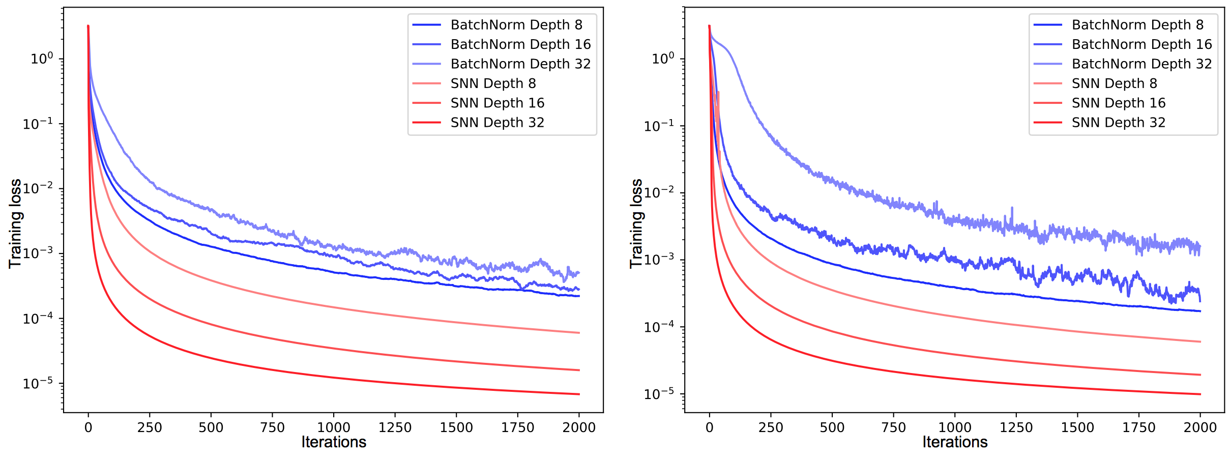
Figure 1. The training error (y-axis) on left: MNIST, right: CIFAR-10. FNN with bn exhibit high variance due to perturbations.
Self-Normalizing Neural Networks (SNNs)
Normalization and SNNs
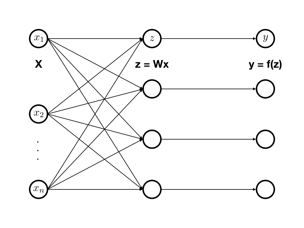
- activation function: $f$
- weight matrix: $\bf{W}$
- activations in the lower layer: $\bf{x}$
- network inputs: $\mathbf{z} = \mathbf{W} \mathbf{x}$
- activations in the higher layer: $\mathbf{y} = f(\mathbf{z})$
- activations $\bf{x}, \bf{y}$ and inputs $\bf{z}$ are random variables
Assume
- all activations $x_{i}$
- mean $\mu := \mathbb{E}(x_{i})$ across samples
- $\mathbb{E} := \sum^{N}$: $N$ is a sample size (my notation)
- variance $\nu := \textrm{Var}(x_{i})$
- mean $\mu := \mathbb{E}(x_{i})$ across samples
- That means
- $\mu := \mathbb{E}(x_{1}) = \mathbb{E}(x_{2}) = \cdots = \mathbb{E}(x_{n})$
- $\nu := \textrm{Var}(x_{1}) = \textrm{Var}(x_{2}) = \cdots = \textrm{Var}(x_{n})$
- $\mathbf{x} = (x_{1}, x_{2}, \cdots, x_{n})$
- single activation $y = f(z), z = \mathbf{w}^{T} \mathbf{x}$
- mean $\tilde{\mu} := \mathbb{E}(y)$
- variance $\tilde{\nu} := \textrm{Var}(y)$
Define
- $n$ times the mean of the weight vector
- $\omega := \sum_{i=1}^{n} w_{i}$, for $\mathbf{w} \in \mathbb{R}^{n}$
- $n$ times the second moment of the weight vector
- $\tau := \sum_{i=1}^{n} w_{i}^{2}$, for $\mathbf{w} \in \mathbb{R}^{n}$
mapping $g$
- mapping $g$ keeps $(\mu, \nu)$ and $(\tilde{\mu}, \tilde{\nu})$ close to predefined values, typically $(0, 1)$
- like most normalization techniques: batch, layer, or weight normalization
Notation summary
- relate to activations: $(\mu, \nu, \tilde{\mu}, \tilde{\nu})$
- relate to weight : $(\omega, \tau)$
Definition 1 (Self-normalizing neural net)
A neural network is self-normalizing if it possesses a mapping $g : \Omega \mapsto \Omega$ for each activation $y$ that maps mean and variance from one layer to the next and has a stable and attracting fixed point depending on $(\omega, \tau)$ in $\Omega$. Furthermore, the mean and the variance remain in the domain $\Omega$, that is $g(\Omega) \subseteq \Omega$, where $\Omega = {(\mu, \nu) | \mu \in [\mu_{\textrm{min}}, \mu_{\textrm{max}}], \nu \in [\nu_{\textrm{min}}, \nu_{\textrm{max}}]}$. When iteratively applying the mapping $g$, each point within $\Omega$ converges to this fixed point.
- if both their mean and their variance across samples are within predefined intervals
- then activations are normalized.
Constructing Self-normalizing Neural Networks
- Tow design choices
- the activation function
- the initialization of the weight
Scaled exponential linear units (SELUs)
- negative and positive values for controlling the mean
- saturation regions (derivatives approaching zero) to dampen the variance if it is too large in the lower layer
- a slope larger than one to increase the variance if it is too small in the lower layer
- a continuous curve.
Weight initialization
- propose $\omega = 0$ and $\tau = 1$ for all units in the higher layer
Deriving the Mean and Variance Mapping Function $g$
Assume
- $x_{i}$: independent from each other but share the same mean $\mu$ and variance $\nu$
- $\mu := \mathbb{E}(x_{1}) = \mathbb{E}(x_{2}) = \cdots = \mathbb{E}(x_{n})$
- $\nu := \textrm{Var}(x_{1}) = \textrm{Var}(x_{2}) = \cdots = \textrm{Var}(x_{n})$
some calculations
- $z = \mathbf{w}^{T} \mathbf{x} = \sum_{i=1}^{n} w_{i} x_{i}$
- $\mathbb{E}(z) = \mathbb{E}( \sum_{i=1}^{n} w_{i} x_{i} ) = \sum_{i=1}^{n} w_{i} \mathbb{E}(x_{i}) = \mu \omega$
- independent summation across dimension $(\sum^{n})$ and summation across samples $(\sum^{N})$
- $\textrm{Var}(z) = \textrm{Var}( \sum_{i=1}^{n} w_{i} x_{i} ) = \nu \tau$
- used the independence of the $x_{i}$
- $\mathbb{E}(z) = \mathbb{E}( \sum_{i=1}^{n} w_{i} x_{i} ) = \sum_{i=1}^{n} w_{i} \mathbb{E}(x_{i}) = \mu \omega$
- Central limit theorem (CLT)
- input $z$ is a weighted sum of i.i.d. variables $x_{i}$
- $z$ approaches a normal distribution
- $z \sim \mathcal{N} (\mu \omega, \sqrt{\nu \tau})$ with density $p_{N}(z; \mu \omega, \sqrt{\nu \tau})$
mapping $g$
calculation of $g$
Remind SELUs
integration
analytic form $\mu$ and $\nu$
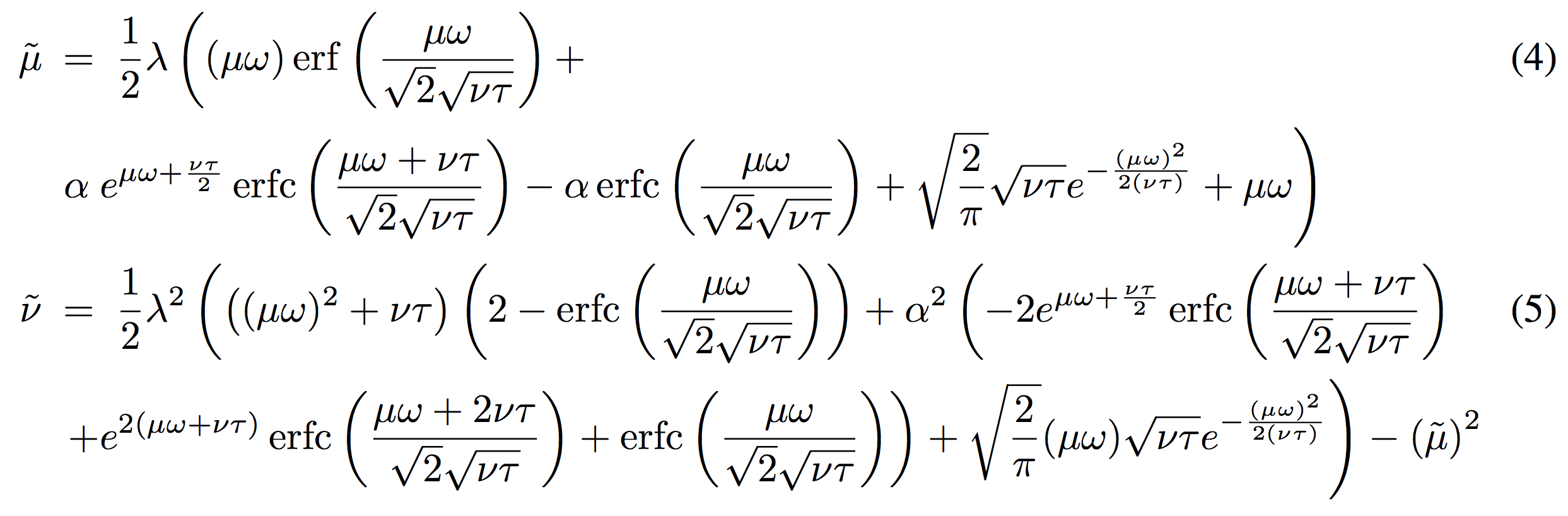
error function
complementary error function
Stable and Attracting Fixed Point $(0, 1)$ for Normalized Weights
Assume
- $\mathbf{w}$ with $\omega = 0$ and $\tau = 1$
- choose a fixed point $(\mu, \nu) = (0, 1)$
- $\mu = \tilde{\mu} = 0$ and $\nu = \tilde{\nu} = 1$
Jacobian of $g$
useful calculations
- $\mu = \tilde{\mu} = 0$ and $\nu = \tilde{\nu} = 1$
- $\omega = 0$ and $\tau = 1$
- $\textrm{erf}(0) = 0$ and $\textrm{erfc}(0) = 1$
- $\frac{\textrm{d}}{\textrm{d} x} \textrm{erf}(x) = \frac{2}{\sqrt{\pi}} e^{-x^{2}}$
- $\left. \frac{\textrm{d}}{\textrm{d} x} \textrm{erf}(x) \right|_{x=0} = \frac{2}{\sqrt{\pi}}$
- $\frac{\textrm{d}}{\textrm{d} x} \textrm{erfc}(x) = \frac{\textrm{d}}{\textrm{d} x} (1 - \textrm{erf}(x))
= - \frac{\textrm{d}}{\textrm{d} x} \textrm{erf}(x)$
- $\left. \frac{\textrm{d}}{\textrm{d} x} \textrm{erfc}(x) \right|_{x=0} = -\frac{2}{\sqrt{\pi}}$
insert $\mu = \tilde{\mu} = 0$, $\nu = \tilde{\nu} = 1$, $\omega = 0$ and $\tau = 1$ into Eq. (4) and (5)
python code
In [1]: from scipy.special import erfc
In [2]: import math
In [3]: alpha = -math.sqrt(2/math.pi) / (math.exp(0.5) * erfc(1/math.sqrt(2)) - 1)
In [4]: l = math.sqrt(2) / math.sqrt(1 + alpha**2 * (-2 * math.exp(0.5) * erfc(1/math.sqrt(2)) + math.exp(2) * erfc(2/math.sqrt(2)) + 1))
In [5]: alpha
Out[5]: 1.6732632423543778
In [6]: l
Out[6]: 1.0507009873554805
calculation of $\frac{\partial \tilde{\mu}}{\partial \mu}$
blackboard
calculation of $\frac{\partial \tilde{\mu}}{\partial \nu}$
blackboard
To be continued
아직 정리가 덜 됐습니다. 조만간 정리해서 올리도록 하겠습니다.
References
-
Ioffe, S. and Szegedy, C. (2015). Batch normalization: Accelerating deep network training by reducing internal covariate shift. In Proceedings of The 32nd International Conference on Machine Learning, pages 448–456. ↩
-
Ba, J. L., Kiros, J. R., and Hinton, G. (2016). Layer normalization. arXiv preprint arXiv:1607.06450. ↩
-
Salimans, T. and Kingma, D. P. (2016). Weight normalization: A simple reparameterization to accelerate training of deep neural networks. In Advances in Neural Information Processing Systems, pages 901–909. ↩
Comments